Common Use Cases

DataServer

The gplately.DataServer class allows users to automatically download and cache the plate reconstruction model files to a designated folder on your system. These files include rotation models, topology features, and static geometries such as coastlines, continents, and continent-ocean boundaries. Additionally, it supports the retrieval of other data types, including rasters, grids, and feature data.

The plate-model-manager Python package is a newly developed alternative to the gplately.DataServer class. Users are encouraged to use the newer plate-model-manager whenever possible.

See also

plate-model-manager documentation

from gplately import DataServer

data_server = DataServer("Muller2019")

# Download plate reconstruction files and geometries from the Müller et al. 2019 model
rotation_model, topology_features, static_polygons = (
   data_server.get_plate_reconstruction_files()
)
coastlines, continents, COBs = data_server.get_topology_geometries()

# Download the age grid at 100Ma from the Müller et al. 2019 model
age_grid = data_server.get_age_grid(times=100)

# Download the ETOPO1 geotiff raster
etopo = data_server.get_raster("ETOPO1_tif")

The table below provides a list of all available plate reconstruction models.

Note

• Use horizontal scrolling to see all the columns in the table.

• All models include rotation data.

Plate Reconstruction Models

Model Name	Topology	Static Polygons	Coasts	Continents	COB	Age Grids	SR Grids
Shirmard2025	✅	✅	✅	✅	✅	❌	❌
Alfonso2024	✅	✅	✅	✅	❌	❌	❌
Cao2024	✅	✅	✅	✅	✅	❌	❌
Muller2022	✅	✅	✅	✅	✅	❌	❌
Zahirovic2022	✅	✅	✅	✅	❌	✅	✅
Merdith2021	✅	✅	✅	✅	❌	❌	❌
Clennett2020	✅	✅	✅	❌	❌	✅	✅
Clennett2020_M2019	✅	✅	✅	❌	❌	✅	✅
Clennett2020_S2013	✅	✅	✅	❌	❌	❌	❌
Muller2019	✅	✅	✅	✅	✅	✅	❌
Young2018	✅	✅	✅	✅	❌	❌	❌
TorsvikCocks2017	❌	✅	✅	❌	❌	❌	❌
Matthews2016	✅	✅	✅	✅	❌	❌	❌
Matthews2016_pmag_ref	❌	✅	✅	✅	❌	❌	❌
Muller2016	✅	✅	✅	❌	✅	✅	❌
Scotese2016	❌	✅	✅	❌	❌	❌	❌
Zahirovic2016	✅	✅	✅	✅	❌	❌	❌
Gibbons2015	✅	✅	✅	❌	❌	❌	❌
Zahirovic2014	❌	✅	✅	❌	❌	❌	❌
Shephard2013	✅	✅	✅	❌	❌	❌	❌
Gurnis2012	✅	✅	✅	❌	❌	❌	❌
Seton2012	✅	✅	✅	✅	✅	✅	❌
Muller2008	❌	✅	❌	❌	❌	❌	❌

Note

• Topology: topological plate polygons and plate boundaries

• Coasts: coastlines. The Greenland coastline uses the Danish Geological Survey dataset. The rest of the world uses the World Vector Shoreline from the the Global Self-consistent Hierarchical High-resolution Geography (GSHHG) dataset.

• Continents: continental polygons, derived from the Static Polygons, containing continental crust and volcanically-modified oceanic crust (including island arcs).

• COB: continent-ocean boundary. The COBs are represented as lines along passive margins and does not include data from active margins.

• Age Grids: numerical grid of seafloor age

• SR Grids: numerical grid of seafloor spreading rate

PlateReconstruction

The gplately.PlateReconstruction class contains tools to reconstruct geological features like tectonic plates and plate boundaries, and to interrogate plate kinematic data like plate motion velocities, and rates of subduction and seafloor spreading.

from gplately import PlateReconstruction, PlateModelManager

model = PlateModelManager().get_model("Muller2019")

# Build a plate reconstruction model using a rotation model, a set of topology features and static polygons
recon_model = PlateReconstruction(
   model.get_rotation_model(),
   topology_features=model.get_layer("Topologies"),
   static_polygons=model.get_layer("StaticPolygons"),
)

Alternatively, you may use the auxiliary functions to create a gplately.PlateReconstruction object.

from gplately.auxiliary import get_plate_reconstruction

# use the auxiliary function to create a PlateReconstruction object
plate_reconstruction_instance = get_plate_reconstruction("Muller2019")

The PlateReconstructions example demonstrates in details how to use the gplately.PlateReconstruction class. The 02-PlateReconstructions.ipynb Jupyter Notebook is available in the GitHub GPlately repository.

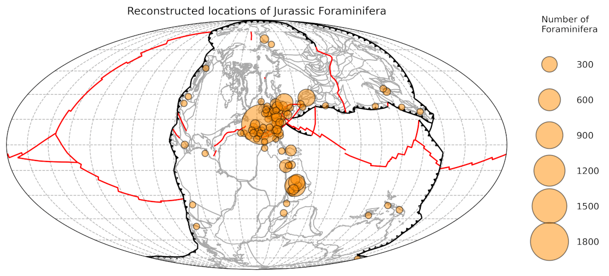
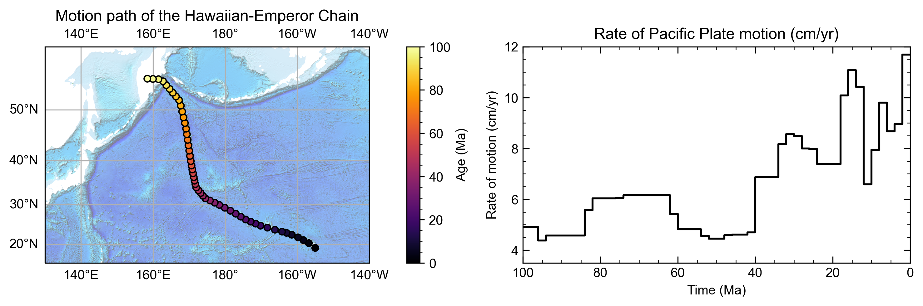
Points

The methods in the gplately.Points class track the motion of a point (or group of points) represented by a latitude and longitude through geologic time. This motion can be visualised using flowlines or motion paths and quantified with point motion velocities.

import numpy as np

from gplately import PlateModelManager, Points, auxiliary

model = PlateModelManager().get_model("Muller2019")

# Create a plate reconstruction model using a rotation model, a set of topology features and static polygons
recon_model = auxiliary.get_plate_reconstruction(model)

# Define some points using their latitude and longitude coordinates so we can track them though time!
pt_lons = np.array([140.0, 150.0, 160.0])
pt_lats = np.array([-30.0, -40.0, -50.0])

# Create a Points object from these points
gpts = Points(recon_model, pt_lons, pt_lats)

The WorkingWithPoints example demonstrates in details how to use the Points class. The 03-WorkingWithPoints.ipynb Jupyter Notebook is available in the GitHub GPlately repository.

The CreatingMotionPathsAndFlowlines example demonstrates how to create motion paths and flowlines. The 09-CreatingMotionPathsAndFlowlines.ipynb Jupyter Notebook is available in the GitHub GPlately repository.

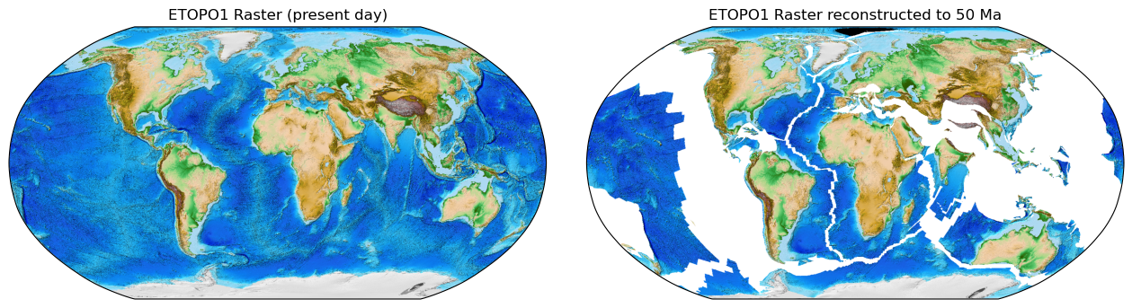
Raster

The gplately.Raster class contains methods to work with netCDF4 or MaskedArray gridded data. Grids may be filled, resized, resampled, and reconstructed back and forwards through geologic time. Other array data can also be interpolated onto Raster grids.

from gplately import PlateModelManager, PresentDayRasterManager, Raster, auxiliary

model_name = "Muller2019"
# Create a plate reconstruction model using a rotation model, a set of topology features and static polygons
recon_model = auxiliary.get_plate_reconstruction(model_name)

# Any numpy array can be turned into a Raster object!
raster = Raster(
   plate_reconstruction=recon_model,
   data=PresentDayRasterManager().get_raster("topography"),
   extent="global",  # equivalent to (-180, 180, -90, 90)
   origin="lower",  # or set extent to (-180, 180, -90, 90)
)

# Reconstruct the raster data to 50 million years ago!
reconstructed_raster = raster.reconstruct(
   time=50,
   partitioning_features=PlateModelManager()
   .get_model(model_name)
   .get_layer("ContinentalPolygons"),
)

The Rasters example demonstrates in details how to use the gplately.Raster class. The 06-Rasters.ipynb Jupyter Notebook is available in the GitHub GPlately repository.

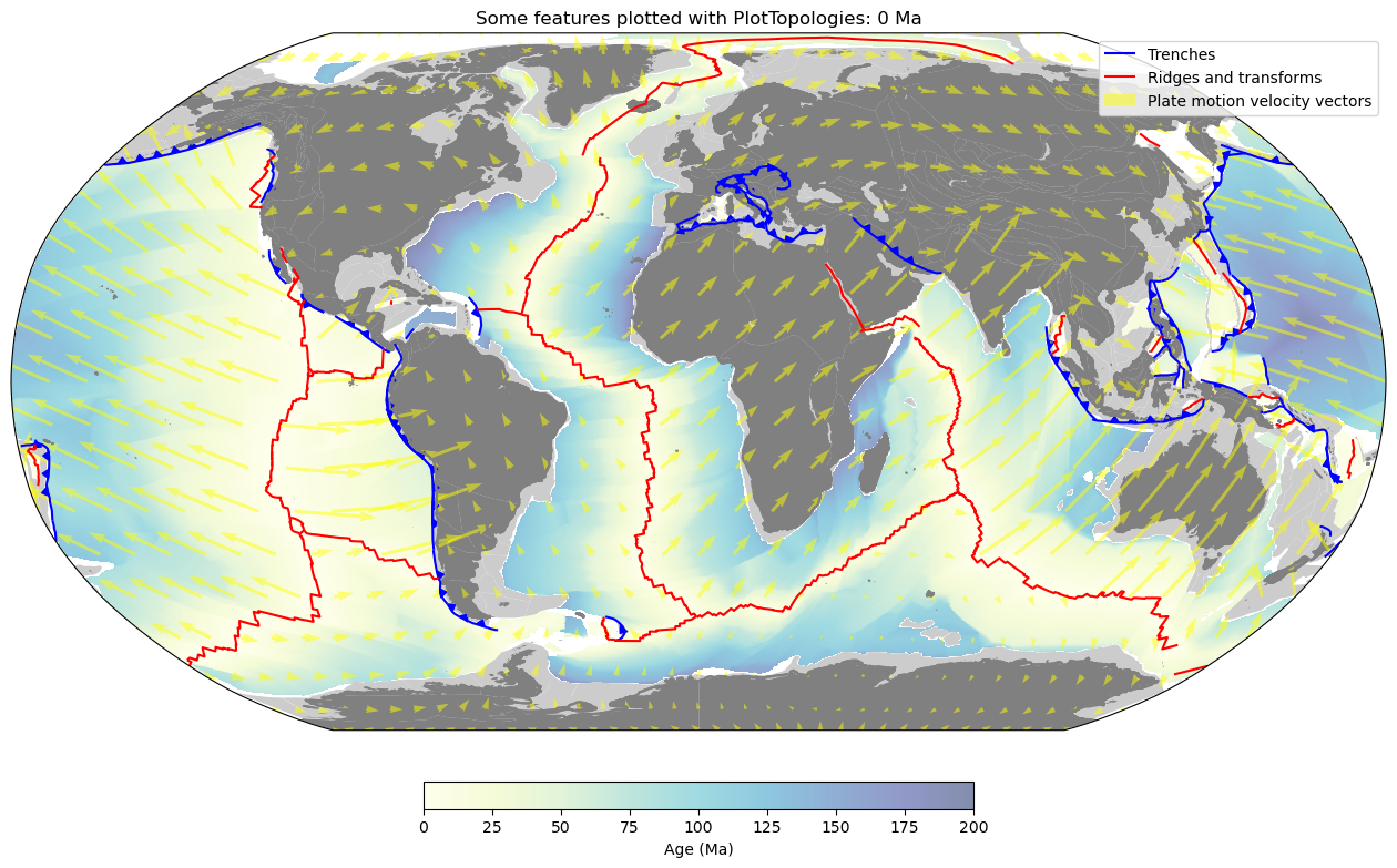
PlotTopologies

The gplately.PlotTopologies class works with the aforementioned gplately.PlateReconstruction class to plot geologic features of different types, such as coastlines, continents and continent-ocean boundaries reconstructed through time using pyGPlates.

from gplately import PlateModelManager, PlotTopologies, auxiliary

model = PlateModelManager().get_model("Muller2019")
recon_model = auxiliary.get_plate_reconstruction(model)

gplot = PlotTopologies(
   recon_model,
   coastlines=model.get_layer("Coastlines"),
   COBs=model.get_layer("COBs"),
   continents=model.get_layer("ContinentalPolygons"),
   time=55,
)

You may use the auxiliary functions to create a gplately.PlotTopologies object.

from gplately.auxiliary import get_gplot

# use the auxiliary function to create a PlotTopologies object
plot_topologies_obj = get_gplot("Muller2019", time=55)

The PlateReconstructions example demonstrates in details how to use the gplately.PlotTopologies class. The 02-PlateReconstructions.ipynb Jupyter Notebook is available in the GitHub GPlately repository.

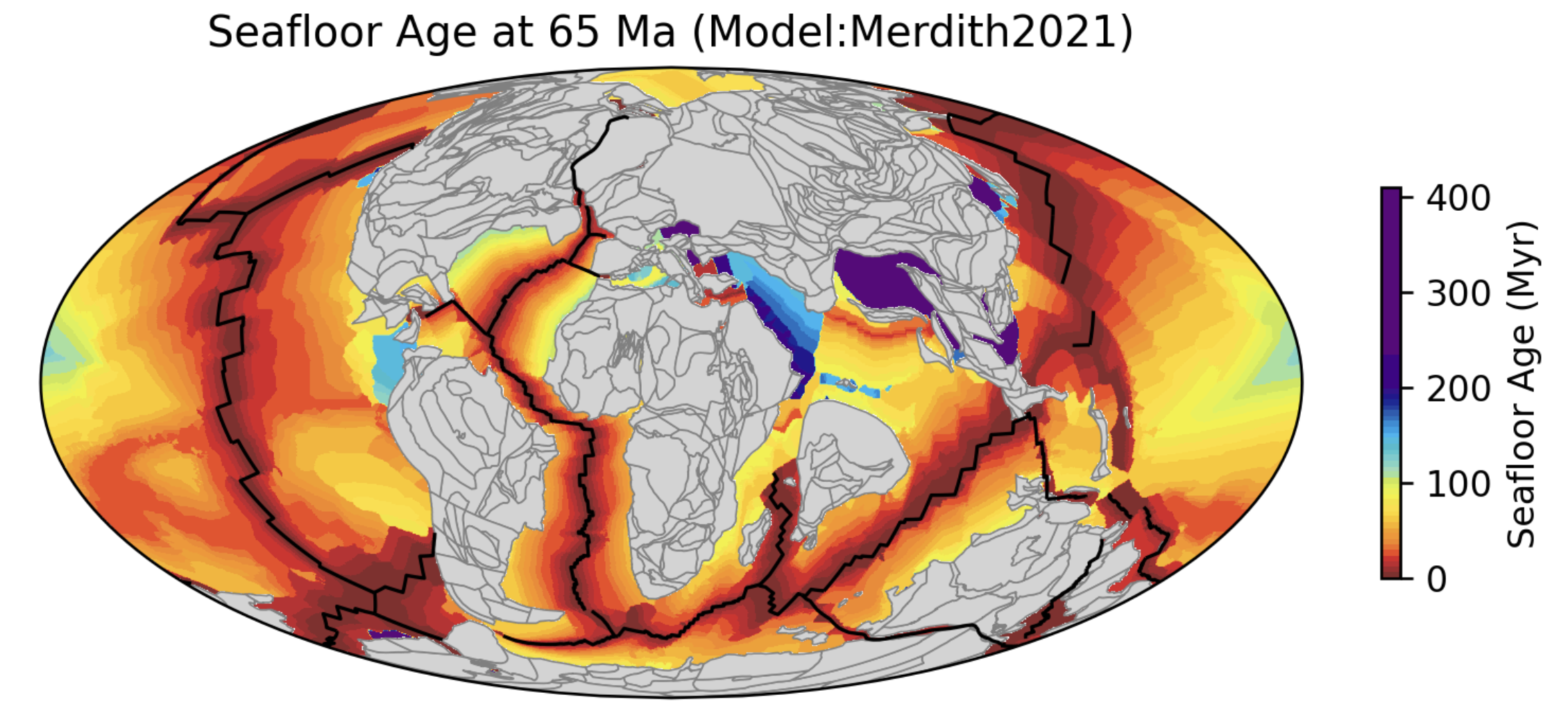
SeafloorGrid

The gplately.SeafloorGrid class wraps an automatic workflow to grid seafloor ages and seafloor spreading rates as encoded by a plate reconstruction model.

import os

os.environ["DISABLE_GPLATELY_DEV_WARNING"] = "true"

from gplately import SeafloorGrid, auxiliary

if __name__ == "__main__":
   gplot = auxiliary.get_gplot("Muller2019")

   # Set up automatic gridding from 5Ma to present day
   seafloorgrid = SeafloorGrid(
      PlateReconstruction_object=gplot.plate_reconstruction,  # The PlateReconstruction object
      PlotTopologies_object=gplot,  # The PlotTopologies object
      max_time=5,  # start time (Ma)
      min_time=0,  # end time (Ma)
      ridge_time_step=1,  # time increment (Myr)
   )

   # Begin automatic gridding!
   seafloorgrid.reconstruct_by_topologies()

The SeafloorGrids example is a tutorial notebook that demonstrates how to set up and use the gplately.SeafloorGrid object, and shows a sample set of output grids. The 10-SeafloorGrids.ipynb Jupyter Notebook is available in the GitHub GPlately repository.