gplately.SeafloorGrid

class gplately.SeafloorGrid(plate_reconstruction, max_time: float | int, min_time: float | int, ridge_time_step: float | int, *, save_directory: str | Path = 'seafloor-grid-output', file_collection: str = '', refinement_levels: int = 6, ridge_sampling: float = 0.5, extent: Tuple = (-180, 180, -90, 90), grid_spacing: float = 0.1, subduction_collision_parameters=(5.0, 10.0), initial_ocean_mean_spreading_rate: float = 75.0, resume_from_checkpoints=False, continent_polygon_features=None, use_continent_contouring=False, continent_mask_filename=None, nprocs=-2)

Bases: object

Generate grids that track data atop global ocean basin points (which emerge from mid-ocean ridges) through geological time.

This generates grids of seafloor age, seafloor spreading rate and other oceanic data from the gplately.PlateReconstruction object. By default, continental polygons are reconstructed to mask out continental regions.

Gridding methods in this class have been adapted from Simon Williams’ development repository for an [auto-age-gridding workflow](https://github.com/siwill22/agegrid-0.1).

The sample jupyter notebook [10-SeafloorGrid](https://github.com/GPlates/gplately/blob/master/Notebooks/10-SeafloorGrids.ipynb) demonstrates how the functionalities within this class work. Below you can find documentation for each of these functionalities.

Methodology

There are two main steps that this class follows to generate grids:

1. Preparation for reconstruction by topologies

2. Reconstruction by topologies

The preparation step involves building a:

• global domain of initial points that populate the seafloor at max_time,

• continental mask that separates ocean points from continent regions per timestep, and

• set of points that emerge to the left and right of mid-ocean ridge segments per timestep, as well as the z-value to allocate to these points.

First, the global domain of initial points is created using [stripy’s](https://github.com/underworldcode/stripy/blob/master/stripy/spherical_meshes.py#L27) icosahedral triangulated mesh. The number of points in this mesh can be controlled using a refinement_levels integer (the larger this integer, the more resolved the initial ocean basin will be).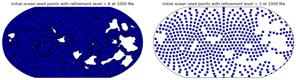


These points are spatially partitioned by plate ID so they can be passed into a point-in-polygon routine. This identifies points that lie within continental polygon boundaries and those that are in the ocean. From this, continental masks are built per timestep, and the initial seed points are allocated ages at the first reconstruction timestep max_time. Each point’s initial age is calculated by dividing its proximity to the nearest MOR segment by half its assumed spreading rate. This spreading rate (initial_ocean_mean_spreading_rate) is assumed to be uniform for all points.

These initial points momentarily fill the global ocean basin, and all have uniform spreading rates. Thus, the spreading rate grid at max_time will be uniformly populated with the initial_ocean_mean_spreading_rate (mm/yr). The age grid at max_time will look like a series of smooth, linear age gradients clearly partitioned by tectonic plates with unique plate IDs: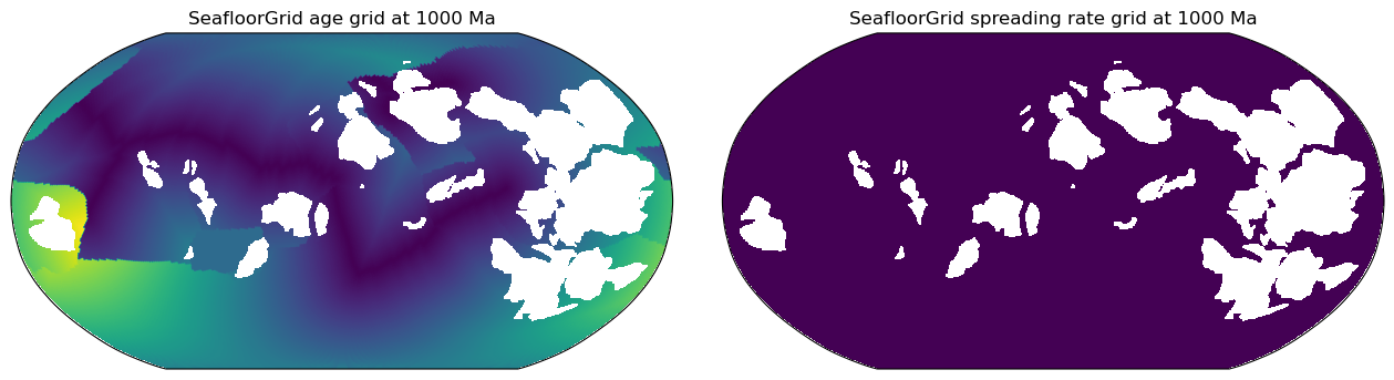


Ridge “line” topologies are resolved at each reconstruction time step and partitioned into segments with a valid stage rotation. Each segment is further divided into points at a specified ridge sampling spacing (ridge_sampling). Each point is ascribed a latitude, longitude, spreading rate and age (from plate reconstruction model files, as opposed to ages of the initial ocean mesh points), a point index and the general z-value that will be gridded onto it.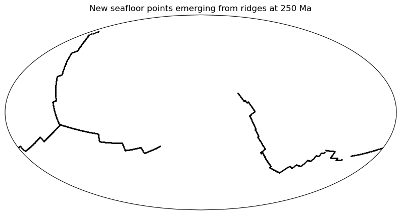


Reconstruction by topologies involves determining which points are active and inactive (collided with a continent or subducted at a trench) for each reconstruction time step. This is done using a hidden object in PlateReconstruction called ReconstructByTopologies.

If an ocean point with a certain velocity on one plate ID transitions into another rigid plate ID at another timestep (with another velocity), the velocity difference between both plates is calculated. The point may have subducted/collided with a continent if this velocity difference is higher than a specified velocity threshold (which can be controlled with subduction_collision_parameters). To ascertain whether the point should be deactivated, a displacement test is conducted. If the proximity of the point’s previous time position to the polygon boundary it is approaching is higher than a set distance threshold, then the point is far enough away from the boundary that it cannot be subducted or consumed by it, and hence the point is still active. Otherwise, it is deemed inactive and deleted from the ocean basin mesh.

With each reconstruction time step, points from mid-ocean ridges (which have more accurate spreading rates and attributed valid times) will spread across the ocean floor. Eventually, points will be pushed into continental boundaries or subduction zones, where they are deleted. Ideally, all initial ocean points (from the Stripy icosahedral mesh) should be deleted over time. However, not all will be deleted - such points typically reside near continental boundaries. This happens if the emerged ridge points do not spread far enough to “phase out” these points at collision regions - likely due to insufficient reconstruction detail. These undeleted points form artefacts of anomalously high seafloor age that append over the reconstruction time range.

Once reconstruction by topologies determines the ocean basin snapshot per timestep, a data frame of all longitudes, latitudes, seafloor ages, spreading rates and any other attributed z values will be written to a gridding input file per timestep.

Each active longitude, latitude and chosen z value is gridded using nearest-neighbour interpolation and written to a netCDF4 format.

__init__(plate_reconstruction, max_time: float | int, min_time: float | int, ridge_time_step: float | int, *, save_directory: str | Path = 'seafloor-grid-output', file_collection: str = '', refinement_levels: int = 6, ridge_sampling: float = 0.5, extent: Tuple = (-180, 180, -90, 90), grid_spacing: float = 0.1, subduction_collision_parameters=(5.0, 10.0), initial_ocean_mean_spreading_rate: float = 75.0, resume_from_checkpoints=False, continent_polygon_features=None, use_continent_contouring=False, continent_mask_filename=None, nprocs=-2)

Constructor. Create a SeafloorGrid object.

Parameters:

• plate_reconstruction (PlateReconstruction) –

  A PlateReconstruction object to provide the following essential components for seafloor gridding.

  • PlateReconstruction.rotation_model

  • PlateReconstruction.topology_featues

• max_time (float) – The maximum time for age gridding.

• min_time (float) – The minimum time for age gridding.

• ridge_time_step (float) – The delta time for resolving ridges (and thus age gridding).

• save_directory (str, default=None) – The top-level directory to save all outputs to.

• file_collection (str, default="") – A string to identify the plate model used (will be automated later).

• refinement_levels (int, default=6) – Control the number of points in the icosahedral mesh (higher integer means higher resolution of initial ocean basin).

• ridge_sampling (float, default=0.5) – Spatial resolution (in degrees) at which points that emerge from ridges are tessellated.

• extent (tuple of 4, default=(-180.,180.,-90.,90.)) – A tuple containing the mininum longitude, maximum longitude, minimum latitude and maximum latitude extents for all masking and final grids.

• grid_spacing (float, default=0.1) – The degree spacing/interval with which to space grid points across all masking and final grids. If grid_spacing is provided, all grids will use it. If not, grid_spacing defaults to 0.1.

• subduction_collision_parameters (len-2 tuple of float, default=(5.0, 10.0)) – A 2-tuple of (threshold velocity delta in kms/my, threshold distance to boundary per My in kms/my)

• initial_ocean_mean_spreading_rate (float, default=75.) – A spreading rate to uniformly allocate to points that define the initial ocean basin. These points will have inaccurate ages, but most of them will be phased out after points with plate-model prescribed ages emerge from ridges and spread to push them towards collision boundaries (where they are deleted).

• resume_from_checkpoints (bool, default=False) – If set to True, and gridding was interrupted in a previous run, then SeafloorGrids will resume gridding. All other parameters and input data should remain unchanged when resuming (otherwise the results will be indeterminate). If set to False, SeafloorGrids will start gridding from scratch.

• continent_polygon_features (str/os.PathLike, or a sequence (eg, list or tuple) of instances of pygplates.Feature, or a single instance of pygplates.Feature, or an instance of pygplates.FeatureCollection, or a sequence of any combination of those four types, optional) – Note that this is ignored if continent_mask_filename is specified, otherwise this argument must be specified. These are the continental polygon or COB terrane polygon features to mask the seafloor grids with. Can be provided as a continental polygon filename, or a sequence of continental polygon features, or a single continental polygon feature, or a continental polygon feature collection, or a sequence (eg, a list or tuple) of any combination of those four types.

• use_continent_contouring (bool, default=False) – Note that this is ignored if continent_mask_filename is specified. If True then builds the continent mask for a given time using ptt’s ‘continent contouring’ method (for more information about ‘Continent Contouring’, visit https://github.com/EarthByte/continent-contouring). If False then builds the continent masks using the continents of continent_polygon_features.

• continent_mask_filename (str, optional) – An optional parameter pointing to the full path to a continental mask for each timestep. Assuming the time is in the filename, i.e. /path/to/continent_mask_0Ma.nc, it should be passed as /path/to/continent_mask_{}Ma.nc with curly brackets. Include decimal formatting if needed.

• nprocs (int, default=-2) – The number of CPUs to use for parts of the code that are parallelized. Must be an integer or convertible to an integer (eg, float is rounded towards zero). If positive then uses that many CPUs. If 1 then executes in serial (ie, is not parallelized). If 0 then a ValueError is raised. If -1 then all available CPUs are used. If -2 then all available CPUs except one are used, etc. Defaults to -2 (ie, uses all available CPUs except one to keep system responsive).

Methods

__init__(plate_reconstruction, max_time, ...)	Constructor.
lat_lon_z_to_netCDF(zval_name[, time_arr, ...])	Produce a netCDF4 grid of a z-value identified by its zval_name for a given time range in time_arr.
reconstruct_by_topological_model()	Use pygplates.TopologicalModel class to reconstruct seed points.
reconstruct_by_topologies()	Obtain all active ocean seed points which are points that have not been consumed at subduction zones or have not collided with continental polygons.

Attributes

CURRENT_LATITUDES_KEY
CURRENT_LONGITUDES_KEY
SEAFLOOR_AGE_KEY
SPREADING_RATE_KEY
max_time	The maximum time for age gridding.

CURRENT_LATITUDES_KEY = 'CURRENT_LATITUDES'

CURRENT_LONGITUDES_KEY = 'CURRENT_LONGITUDES'

SEAFLOOR_AGE_KEY = 'SEAFLOOR_AGE'

SPREADING_RATE_KEY = 'SPREADING_RATE'

lat_lon_z_to_netCDF(zval_name, time_arr=None, unmasked=False, nprocs=None)

Produce a netCDF4 grid of a z-value identified by its zval_name for a given time range in time_arr.

Seafloor age can be gridded by passing zval_name as SEAFLOOR_AGE, and spreading rate can be gridded with SPREADING_RATE.

Saves all grids to compressed netCDF format in the attributed directory. Grids can be read into ndarray format using gplately.read_netcdf_grid().

Parameters:

• zval_name (str) – A string identifier for the z-value.

• time_arr (list of float, default=None) – A time range to turn lons, lats and z-values into netCDF4 grids. If not provided, time_arr defaults to the full time_array provided to SeafloorGrid.

• unmasked (bool, default=False) – Save unmasked grids, in addition to masked versions.

• nprocs (int, optional) – Optional number of CPUs to use for producing grids. If not specified then defaults to the number of CPUs specified in __init__(). If specified then must be an integer or convertible to an integer (eg, float is rounded towards zero). If positive then uses that many CPUs. If 1 then executes in serial (ie, is not parallelized). If 0 then a ValueError is raised. If -1 then all available CPUs are used. If -2 then all available CPUs except one are used, etc.

property max_time

The maximum time for age gridding.

Type:

float

reconstruct_by_topological_model()

Use pygplates.TopologicalModel class to reconstruct seed points. This method is an alternative to reconstruct_by_topologies() which uses Python code to do the reconstruction.

reconstruct_by_topologies()

Obtain all active ocean seed points which are points that have not been consumed at subduction zones or have not collided with continental polygons. Active points’ latitudes, longitues, seafloor ages, spreading rates and all other general z-values are saved to a gridding input file (.npz).