Rule Based GPML Processing Pipeline
This notebook demonstrates how to use GPlately to query and manipulate GPML files based on user-defined rules, which can be based on various criteria such as feature name, plate ID, birth age, disappearance age, region of interest, and more. This allows users to create customized GPML processing pipelines that can be applied to a wide range of use cases in geoscience research.
Built-in feature filters and transformers are available in GPlately to facilitate the creation of custom processing pipelines. For more information, see the documentation for each filter and transformer class.
Download test GPML files and load them as pygplates FeatureCollection objects.
from pathlib import Path
from os.path import exists
from urllib.request import urlretrieve
import matplotlib.pyplot as plt
import cartopy.crs as ccrs

import pygplates

from gplately.utils.feature_filter import (
    FeatureFilter,
    EndTimeFilter,
    FeatureIDFilter,
    FeatureNameFilter,
    PlateIDFilter,
    BirthAgeFilter,
    FeatureTypeFilter,
    PolygonAreaFilter,
    PropertyExistsFilter,
    PropertyValueFilter,
    RegionOfInterestFilter,
    TopologicalFeaturesWithDuplicateSectionsFilter,
    TopologicalReferenceFilter,
    filter_feature_collection,
)
from gplately.plot import cartopy_plot

from gplately.gpml import (
    FeatureCollectionProcessor,
    gpml_to_pandas_dataframe,
    merge_feature_collections,
)
from gplately.utils.feature_transformer import (
    SetReconstructionPlateIDTransformer,
    SetValidTimeTransformer,
)

data_dir = Path("WorkflowData/14-Rule-Based-GPML-Processing-Pipeline")
data_dir.mkdir(parents=True, exist_ok=True)

# Download the test feature collection files if they do not exist.
test_files = [
    (
        "https://repo.gplates.org/webdav/mchin/data/Global_EarthByte_GPlates_PresentDay_Coastlines.gpmlz",
        f"{data_dir}/Global_EarthByte_GPlates_PresentDay_Coastlines.gpmlz",
    ),
    (
        "https://repo.gplates.org/webdav/mchin/data/Feature_Geometries.gpmlz",
        f"{data_dir}/Feature_Geometries.gpmlz",
    ),
    (
        "https://repo.gplates.org/webdav/mchin/data/Plate_Boundaries.gpmlz",
        f"{data_dir}/Plate_Boundaries.gpmlz",
    ),
]

filepaths = []
for test_file in test_files:
    url, file_path = test_file
    if not exists(file_path):
        print(f"Downloading test file to {file_path}...")
        urlretrieve(url, file_path)
    filepaths.append(file_path)

coastlines_feature_collection, topology_feature_collection, boundary_feature_collection = pygplates.FeatureCollection().read(filepaths)

subduction_polarity_left = pygplates.Enumeration(
    pygplates.EnumerationType.create_gpml("SubductionPolarityEnumeration"), "Left"
)
print(f"Finished preparation of running this notebook.")
Matplotlib is building the font cache; this may take a moment.
Downloading test file to WorkflowData/14-Rule-Based-GPML-Processing-Pipeline/Global_EarthByte_GPlates_PresentDay_Coastlines.gpmlz...
Downloading test file to WorkflowData/14-Rule-Based-GPML-Processing-Pipeline/Feature_Geometries.gpmlz...
Downloading test file to WorkflowData/14-Rule-Based-GPML-Processing-Pipeline/Plate_Boundaries.gpmlz...
Finished preparation of running this notebook.
Search and filter feature collection with pre-defined filters
Pre-defined filters:
- FeatureNameFilter: filter features based on their names, with options for exact match, case sensitivity, and exclusion.
- PlateIDFilter: filter features based on their plate IDs, with an option for exclusion.
- BirthAgeFilter: filter features based on their birth ages, with an option to keep features that are older or younger than a specified age.
- FeatureTypeFilter: filter features based on their feature types.
- PropertyExistsFilter: filter features based on the existence of a specified property, with an option for excluding features that have the property.
- PropertyValueFilter: filter features based on the value of a specified property, with an option for excluding features that match the specified value.
- EndTimeFilter: filter features based on their disappearance ages, with options to keep features that disappeared before or after a specified age.
Examples:
- case 1: Search features whose name contains "Australia", "New Zealand" or "Tasmania".
- case 2: Filter out features whose name contains "Australia", "New Zealand" or "Tasmania" from the global coastlines.
- case 3: Search features whose plate ID is from 701 to 715, which correspond to the Africa and its neighboring plates.
- case 4: Filter out features whose plate ID is from 701 to 715 from the global coastlines.
- case 5: Search features whose birth ages are older than 500 million years.
- case 6: Search features whose birth ages are younger than 500 million years.
- case 7: Search features whose feature type is gpml:Basin or gpml:IslandArc.
- case 8: Search features with gpml:subductionPolarity property.
- case 9: Search features whose gpml:subductionPolarity is "Left".
- case 10: Search features that had disappeared 100 million years ago.
- case 11: Search features that still exist at present day.
📒 The results of case 10 and 11 are not plotted because they are time-dependent. You can open the output files in GPlates desktop software to check the results. You will see there is no feature after 100 Myr in the output file of case 10 and there are only features that still exist at present day in the output file of case 11.
fig = plt.figure(figsize=(16, 8), dpi=72)
ax1 = fig.add_subplot(331, projection=ccrs.Robinson(central_longitude=180))
ax2 = fig.add_subplot(332, projection=ccrs.Robinson(central_longitude=180))
ax3 = fig.add_subplot(333, projection=ccrs.Robinson(central_longitude=0))
ax4 = fig.add_subplot(334, projection=ccrs.Robinson(central_longitude=0))
ax5 = fig.add_subplot(335, projection=ccrs.Robinson(central_longitude=0))
ax6 = fig.add_subplot(336, projection=ccrs.Robinson(central_longitude=0))
ax7 = fig.add_subplot(337, projection=ccrs.Robinson(central_longitude=0))
ax8 = fig.add_subplot(338, projection=ccrs.Robinson(central_longitude=0))
ax9 = fig.add_subplot(339, projection=ccrs.Robinson(central_longitude=0))

cases = []
# case 1: features whose name contains "Australia", "New Zealand" or "Tasmania" will be saved in the output file.
cases.append(
    {
        "title": "Coastlines of Australia",
        "feature_collection": coastlines_feature_collection,
        "filters": [
            FeatureNameFilter(
                ["Australia", "New Zealand", "Tasmania"],
                exact_match=False,
                case_sensitive=True,
            )
        ],
        "output_file": f"{data_dir}/Australia_and_New_Zealand_coastlines.gpmlz",
        "ax": ax1,
    }
)
# case 2: features whose name contains "Australia", "New Zealand" or "Tasmania" will be taken out of the global coastlines.
cases.append(
    {
        "title": "Coastlines excluding Australia",
        "feature_collection": coastlines_feature_collection,
        "filters": [
            FeatureNameFilter(
                ["Australia", "New Zealand", "Tasmania"],
                reverse=True,
                exact_match=False,
                case_sensitive=True,
            )
        ],
        "output_file": f"{data_dir}/coastlines_exclude_Australia_and_New_Zealand.gpmlz",
        "ax": ax2,
    }
)
# case 3: features whose plate ID is from 701 to 715, which correspond to the Africa and its neighboring plates, will be saved in the output file.
cases.append(
    {
        "title": "Coastlines of Africa",
        "feature_collection": coastlines_feature_collection,
        "filters": [
            PlateIDFilter(
                list(
                    range(701, 716, 1)
                ),  # This is the list of plate IDs for the Africa and its neighboring plates
                reverse=False,
            )
        ],
        "output_file": f"{data_dir}/coastlines_with_plate_id_from_701_to_715.gpmlz",
        "ax": ax3,
    }
)
# case 4: features whose plate ID is from 701 to 715, which correspond to the Africa and its neighboring plates, will be taken out of the global coastlines.
cases.append(
    {
        "title": "Coastlines excluding Africa",
        "feature_collection": coastlines_feature_collection,
        "filters": [
            PlateIDFilter(
                list(
                    range(701, 716, 1)
                ),  # This is the list of plate IDs for the Africa and its neighboring plates
                reverse=True,  # exclude features with the specified plate IDs
            )
        ],
        "output_file": f"{data_dir}/coastlines_exclude_plate_id_from_701_to_715.gpmlz",
        "ax": ax4,
    }
)

# case 5: features whose birth ages are older than 500 million years will be saved in the output file.
cases.append(
    {
        "title": "Coastlines older than 500 Myr",
        "feature_collection": coastlines_feature_collection,
        "filters": [
            BirthAgeFilter(
                500, reverse=False
            )  # This filter will keep features that were born more than 500 million years ago.
        ],
        "output_file": f"{data_dir}/coastlines_older_than_500_million_years.gpmlz",
        "ax": ax5,
    }
)

# case 6: features whose birth ages are younger than 500 million years will be saved in the output file.
cases.append(
    {
        "title": "Coastlines younger than 500 Myr",
        "feature_collection": coastlines_feature_collection,
        "filters": [
            BirthAgeFilter(
                500, reverse=True
            )  # This filter will keep features that were born less than 500 million years ago.
        ],
        "output_file": f"{data_dir}/coastlines_younger_than_500_million_years.gpmlz",
        "ax": ax6,
    }
)

# case 7: features whose feature type is gpml:Basin or gpml:IslandArc will be saved in the output file.
cases.append(
    {
        "title": "Coastlines with feature type Basin or IslandArc",
        "feature_collection": coastlines_feature_collection,
        "filters": [
            FeatureTypeFilter(
                "gpml:Basin|gpml:IslandArc",
            )
        ],
        "output_file": f"{data_dir}/coastlines_basins_and_island_arcs.gpmlz",
        "ax": ax7,
    }
)
# case 8: features with gpml:subductionPolarity property will be saved in the output file.
cases.append(
    {
        "title": "Topology with subduction polarity",
        "feature_collection": topology_feature_collection,
        "filters": [PropertyExistsFilter("gpml:subductionPolarity", reverse=False)],
        "output_file": f"{data_dir}/topology_with_subduction_polarity.gpmlz",
        "ax": ax8,
    }
)

# case 9: features whose gpml:subductionPolarity is "Left" will be saved in the output file.
cases.append(
    {
        "title": "Topology with subduction polarity of Left",
        "feature_collection": topology_feature_collection,
        "filters": [
            PropertyValueFilter(
                "gpml:subductionPolarity", subduction_polarity_left, reverse=False
            )
        ],
        "output_file": f"{data_dir}/topology_with_subduction_polarity_left.gpmlz",
        "ax": ax9,
    }
)

# case 10: features that had disappeared before 100 million years ago will be saved in the output file.
cases.append(
    {
        "title": "Topology features that had disappeared before 100 Ma",
        "feature_collection": topology_feature_collection,
        "filters": [EndTimeFilter(100, reverse=False)],
        "output_file": f"{data_dir}/topology_features_disappeared_before_100_million_years.gpmlz",
        "ax": None,  # no plot for this case
    }
)

# case 11: features that still exist at present day will be saved in the output file.
cases.append(
    {
        "title": "Topology features that still exist at present day",
        "feature_collection": topology_feature_collection,
        "filters": [EndTimeFilter(0, reverse=True)],
        "output_file": f"{data_dir}/topology_features_still_existing_present_day.gpmlz",
        "ax": None,  # no plot for this case
    }
)

idx = 0
for case in cases:
    idx += 1
    features = filter_feature_collection(
        case["feature_collection"],
        case["filters"],
    )

    features.write(case["output_file"])  # type: ignore
    print(f"\"{case['title']}\" have been written to {case['output_file']}")

    # plot the output feature collection to check if the search worked as expected.
    if case["ax"] is not None:
        # we only plot the features that still exist at present day for better visualization.
        present_day_features = filter_feature_collection(
            pygplates.FeatureCollection(  # type: ignore
                case["output_file"],
            ),
            [EndTimeFilter(0, reverse=True)],
        )
        cartopy_plot._plot_feature_collection(
            present_day_features,
            title=f"Fig {idx}: {case['title']}",
            ax=case["ax"],
            add_gridlines=True,
        )

plt.tight_layout()
plt.show()
"Coastlines of Australia" have been written to WorkflowData/14-Rule-Based-GPML-Processing-Pipeline/Australia_and_New_Zealand_coastlines.gpmlz
"Coastlines excluding Australia" have been written to WorkflowData/14-Rule-Based-GPML-Processing-Pipeline/coastlines_exclude_Australia_and_New_Zealand.gpmlz
"Coastlines of Africa" have been written to WorkflowData/14-Rule-Based-GPML-Processing-Pipeline/coastlines_with_plate_id_from_701_to_715.gpmlz
"Coastlines excluding Africa" have been written to WorkflowData/14-Rule-Based-GPML-Processing-Pipeline/coastlines_exclude_plate_id_from_701_to_715.gpmlz
"Coastlines older than 500 Myr" have been written to WorkflowData/14-Rule-Based-GPML-Processing-Pipeline/coastlines_older_than_500_million_years.gpmlz
"Coastlines younger than 500 Myr" have been written to WorkflowData/14-Rule-Based-GPML-Processing-Pipeline/coastlines_younger_than_500_million_years.gpmlz
"Coastlines with feature type Basin or IslandArc" have been written to WorkflowData/14-Rule-Based-GPML-Processing-Pipeline/coastlines_basins_and_island_arcs.gpmlz
"Topology with subduction polarity" have been written to WorkflowData/14-Rule-Based-GPML-Processing-Pipeline/topology_with_subduction_polarity.gpmlz
"Topology with subduction polarity of Left" have been written to WorkflowData/14-Rule-Based-GPML-Processing-Pipeline/topology_with_subduction_polarity_left.gpmlz
"Topology features that had disappeared before 100 Ma" have been written to WorkflowData/14-Rule-Based-GPML-Processing-Pipeline/topology_features_disappeared_before_100_million_years.gpmlz
"Topology features that still exist at present day" have been written to WorkflowData/14-Rule-Based-GPML-Processing-Pipeline/topology_features_still_existing_present_day.gpmlz

Use Pandas DataFrame to filter features
The code cell below demonstrates how to use the gpml_to_pandas_dataframe function to convert
a GPML feature collection to a Pandas DataFrame, and then use the DataFrame to
filter features based on their properties.
In this example, we filter features whose name contains "Africa" and then check if
the filtered features are correct by comparing the feature IDs of the filtered features with
the feature IDs obtained from the DataFrame filtering.
gdf = gpml_to_pandas_dataframe(coastlines_feature_collection)
# use pandas dataframe to filter features whose name contains the specified name, and get the feature IDs of the filtered features.
africa_feature_ids = gdf[
    gdf["name"].str.contains("Africa", case=False, na=False)
].index.tolist()

feature_id_filter = FeatureIDFilter(africa_feature_ids)

features_with_name_africa = filter_feature_collection(
    coastlines_feature_collection,
    [feature_id_filter],
)

# assert the list of filtrate features is in the same order as the list of given feature IDs.
# use filtrate_features_as_list to get the list of filtered features in the same order as the given feature IDs.
for fid, feature in zip(
    africa_feature_ids, feature_id_filter.filtrate_features_as_list
):
    assert (
        feature is not None
    ), f"Feature with ID {fid} is not found in the feature collection."
    assert (
        fid == feature.get_feature_id().get_string()
    ), f"Feature ID mismatch: {fid} != {feature.get_feature_id().get_string()}"

print(
    f"There are {len(features_with_name_africa)} out of {len(coastlines_feature_collection)} features whose name contains 'Africa' in the global coastlines feature collection."
)
There are 77 out of 2077 features whose name contains 'Africa' in the global coastlines feature collection.
Search feature collection with a user defined filter and update the filtrate features with a transformer
There are some features in the topology feature collection whose "end time" is 0, which should be "distant future" instead, unless some major geological events will happen soon to destroy them.
The code cell below demonstrates how to create a filter by subclassing the FeatureFilter class,
and then use this filter to search a feature collection and update the filtered features' "end time" to "distant future".
# define a filter that finds all features with "end time" equal to 0
class ZeroEndTimeFilter(FeatureFilter):
    def should_keep(self, feature: pygplates.Feature) -> bool:  # type: ignore
        valid_time = feature.get_valid_time(None)
        if valid_time:
            if valid_time[1] == 0:
                return True
        return False


# update the "end time" to "distant future" for features with "end time" equal to 0
updated_feature_collection = FeatureCollectionProcessor(
    filters=[ZeroEndTimeFilter()],
    transformers=[
        SetValidTimeTransformer(
            end_time=pygplates.GeoTimeInstant.create_distant_future()  # pyright: ignore[reportAttributeAccessIssue]
        )
    ],
).process(topology_feature_collection)

print(
    f"{len(updated_feature_collection)} features out of {len(topology_feature_collection)} were updated. Changed end time to distant future for features whose end time was 0."
)
2143 features out of 5165 were updated. Changed end time to distant future for features whose end time was 0.
Find Laurussia topological plate and extract the reference features for investigation
The Laurussia topological plate has duplicate section features. Use its feature ID "GPlates-cfe96235-5906-4974-a654-2b14a260a3fe" to find it. We will find the section features for this topological plate and save them together in a new GPML file for investigation. Open the output file in GPlates desktop software, you will see the Laurussia topological plate at 371 Ma and the section features that are used to construct the topological geometry of this plate.
# get the feature by feature ID
laurussia_371 = filter_feature_collection(
    boundary_feature_collection,
    [FeatureIDFilter(["GPlates-cfe96235-5906-4974-a654-2b14a260a3fe"])],
)

# print some information about the laurussia_371 feature to check if we get the correct feature.
for feature in laurussia_371:
    print(feature.get_feature_id().get_string())
    print(feature.get_valid_time(None))

# get the section features for the Laurussia topological plate
laurussia_371_section_features = filter_feature_collection(
    topology_feature_collection,
    [TopologicalReferenceFilter(laurussia_371)],
)

merge_feature_collections([laurussia_371, laurussia_371_section_features]).write(
    f"{data_dir}/laurussia_371_with_section_features.gpmlz"
)
print(
    f"Laurussia topological boundary and the section features have been written to {data_dir}/laurussia_371_with_section_features.gpmlz"
)
GPlates-cfe96235-5906-4974-a654-2b14a260a3fe
(374.0, 370.1)
Laurussia topological boundary and the section features have been written to WorkflowData/14-Rule-Based-GPML-Processing-Pipeline/laurussia_371_with_section_features.gpmlz
Find all topological boundaries with duplicate section features for investigation
Find all topological boundaries with duplicate section features from a feature collection, and then extract the reference section features for these topological boundaries and save them together in a new GPML file for investigation.
topology_with_duplicated_sections = filter_feature_collection(
    boundary_feature_collection,
    [TopologicalFeaturesWithDuplicateSectionsFilter()],
)

print(
    f"There are {len(topology_with_duplicated_sections)} out of {len(boundary_feature_collection)} features whose topological geometries have duplicate section features."
)

topo_ref_filter = TopologicalReferenceFilter(topology_with_duplicated_sections)
topological_section_features = filter_feature_collection(
    topology_feature_collection,
    [topo_ref_filter],
)

merge_feature_collections(
    [topology_with_duplicated_sections, topological_section_features]
).write(f"{data_dir}/topology_with_duplicate_sections_and_the_section_features.gpmlz")
print(
    f"Topology features with duplicate sections and the section features have been written to {data_dir}/topology_with_duplicate_sections_and_the_section_features.gpmlz"
)
There are 294 out of 2989 features whose topological geometries have duplicate section features.
Topology features with duplicate sections and the section features have been written to WorkflowData/14-Rule-Based-GPML-Processing-Pipeline/topology_with_duplicate_sections_and_the_section_features.gpmlz
Topological reference map
The map of topological feature ID to the list of section feature IDs used in the topological geometries of that topological feature can be accessed by the property "topological_reference_map" of the TopologicalReferenceFilter. The keys of this map are the string representation of the feature IDs of the topological boundary features, and the values are lists of string representation of the feature IDs of the section features used to construct the topological boundaries.
# you will see the length of the topological reference map is the same
# as the number of topological features with duplicate sections
print(len(topo_ref_filter.topological_reference_map))

# now print all the reference section feature IDs for the Laurussia topological plate
print(
    topo_ref_filter.topological_reference_map.get(
        "GPlates-cfe96235-5906-4974-a654-2b14a260a3fe"
    )
)
294
['GPlates-c2d78b11-3ad0-4d1a-876f-d10b41f1de5e', 'GPlates-93dab7ec-8ba9-46a5-8906-cc99d409daed', 'GPlates-4bb297f2-fb36-464e-9ffc-af5f2f9083b8', 'GPlates-8dd2bcb3-7ad7-45ce-95e0-399977ec5846', 'GPlates-026c1975-e56e-4cb9-9320-c6da1c02898c', 'GPlates-ae402c97-a36e-4f47-a9e2-1d9e133698a4', 'GPlates-5067a2fe-34ab-47c0-8eea-a621fffd8b1d', 'GPlates-86e97bb6-65af-4d00-9a8e-cda7f4a879df', 'GPlates-fb98d66d-9b3d-4468-a7bf-a8caaed5dcb8', 'GPlates-4454fcce-c9c0-4e8a-8b2c-e44e9debfbfa', 'GPlates-9e08acc4-a70e-4957-ba21-dd209ea7b2c5', 'GPlates-fb9800fd-2b2b-441e-a8b1-1ad0fdb1522b', 'GPlates-861ecfe3-bcff-42a9-9abc-a26de0de94b5', 'GPlates-fb9800fd-2b2b-441e-a8b1-1ad0fdb1522b', 'GPlates-861ecfe3-bcff-42a9-9abc-a26de0de94b5', 'GPlates-a4915425-66ab-451b-84cd-c0e20f416116']
Find points inside a region of interest
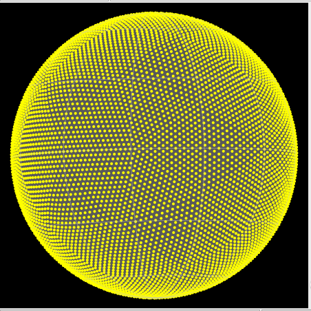
Firstly, we create a feature collection for the vertices of an icosahedron mesh. Then we search for the vertices that are located within a region of interest defined by a bounding box (left, right, bottom, top). Finally, we create a feature for the region of interest and add it to the output feature collection for visualization.
from gplately.lib.icosahedron import get_mesh, xyz2lonlat

# Create a feature collection for the vertices of an icosahedron mesh.
# We will use this feature collection as input for searching features within a region of interest in the next step.
mesh_resolution = 5
vertices_0, faces_0 = get_mesh(mesh_resolution)
seen = set()
mesh_feature_collection = pygplates.FeatureCollection()  # type: ignore
for v in vertices_0:
    lon, lat = xyz2lonlat(v[0], v[1], v[2])
    point = f"{lon:0.2f} {lat:0.2f}"
    if point in seen:
        continue
    else:
        seen.add(point)
    feature = pygplates.Feature()  # type: ignore
    feature.set_geometry(pygplates.PointOnSphere(lat, lon))  # type: ignore
    mesh_feature_collection.add(feature)  # type: ignore

mesh_feature_collection.write(f"{data_dir}/icosahedron_mesh_{mesh_resolution}.gpmlz")
print(
    f"Icosahedron mesh have been written to {data_dir}/icosahedron_mesh_{mesh_resolution}.gpmlz"
)
Icosahedron mesh have been written to WorkflowData/14-Rule-Based-GPML-Processing-Pipeline/icosahedron_mesh_5.gpmlz
if you open the icosahedron_mesh_5.gpmlz file in GPlates, you will see the vertices of the icosahedron mesh, which are represented as point features.
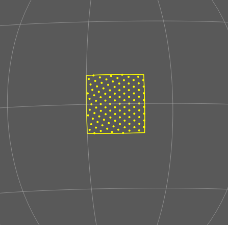
Search for the vertices that are located within a region of interest defined by a bounding box (left, right, bottom, top) in longitude and latitude.
# define the bounding box for the region of interest
left, right, bottom, top = (120, 140, -10, 10)
filters = []
filters.append(RegionOfInterestFilter((left, right, bottom, top), reverse=False))

features = filter_feature_collection(
    mesh_feature_collection,
    filters,
)

# Create a feature for the region of interest and add it to the output feature collection for visualization.
region_of_interest_feature = pygplates.Feature()  # type: ignore
region_of_interest = pygplates.PolygonOnSphere(
    (lat, lon)
    for lon, lat in [
        (left, bottom),
        (left, top),
        (right, top),
        (right, bottom),
        (left, bottom),
    ]
 )  # type: ignore
region_of_interest_feature.set_geometry(region_of_interest)  # type: ignore
features.add(region_of_interest_feature)  # type: ignore

features.write(f"{data_dir}/icosahedron_vertices_in_region.gpmlz")
print(
    f"Icosahedron vertices in the region of interest have been written to {data_dir}/icosahedron_vertices_in_region.gpmlz"
 )
Icosahedron vertices in the region of interest have been written to WorkflowData/14-Rule-Based-GPML-Processing-Pipeline/icosahedron_vertices_in_region.gpmlz
If you open icosahedron_vertices_in_region.gpmlz in GPlates, you will see the vertices of the icosahedron mesh that are located within the bounding box defined by (120, 140, -10, 10), as well as a polygon feature that represents the region of interest defined by the bounding box.
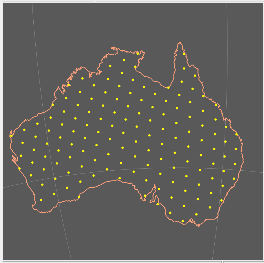
Find the points within the mainland of Australia and set their plate ID to 801.
# Firstly, we search for the feature that corresponds to the mainland of Australia in the global coastline feature collection.
# Then we use the geometry of this feature to define the region of interest for filtering the vertices of the icosahedron mesh.

# find the polygon feature with area greater than 7 million among the features whose name contains "Australia",
# which should correspond to the mainland of Australia, and use its geometry as the region of interest
# for filtering the vertices of the icosahedron mesh.
features = filter_feature_collection(
    coastlines_feature_collection,
    [
        FeatureNameFilter(
            ["Australia"],
            exact_match=True,
            case_sensitive=True,
        ),
        PolygonAreaFilter(7e6, reverse=False),
    ],
)
assert (
    len(features) == 1
), f"Expected to find exactly one feature for the mainland of Australia, but found {len(features)} features."

australia_mainland_feature = features[0]
australia_mainland_geometry = australia_mainland_feature.get_geometry()

##### find the points within the mainland of Australia and set their plate ID to 801.
features = FeatureCollectionProcessor(
    filters=[RegionOfInterestFilter(australia_mainland_geometry, reverse=False)],
    transformers=[SetReconstructionPlateIDTransformer(plate_id=801)],
).process(mesh_feature_collection)

features.add(australia_mainland_feature)  # type: ignore
output_file = f"{data_dir}/icosahedron_vertices_within_australia.gpmlz"
features.write(output_file)
print(
    f"Icosahedron vertices in the region of interest have been written to {output_file}"
)
Icosahedron vertices in the region of interest have been written to WorkflowData/14-Rule-Based-GPML-Processing-Pipeline/icosahedron_vertices_within_australia.gpmlz
If you open icosahedron_vertices_within_australia.gpmlz in GPlates, you will see the vertices of the icosahedron mesh that are located within the mainland of Australia, as well as a polygon feature that represents the mainland of Australia