10 - Seafloor Grids

An adaptation of agegrid-01 written by Simon Williams, Nicky Wright and John Cannon for gridding general z-values onto seafloor basin points using GPlately.

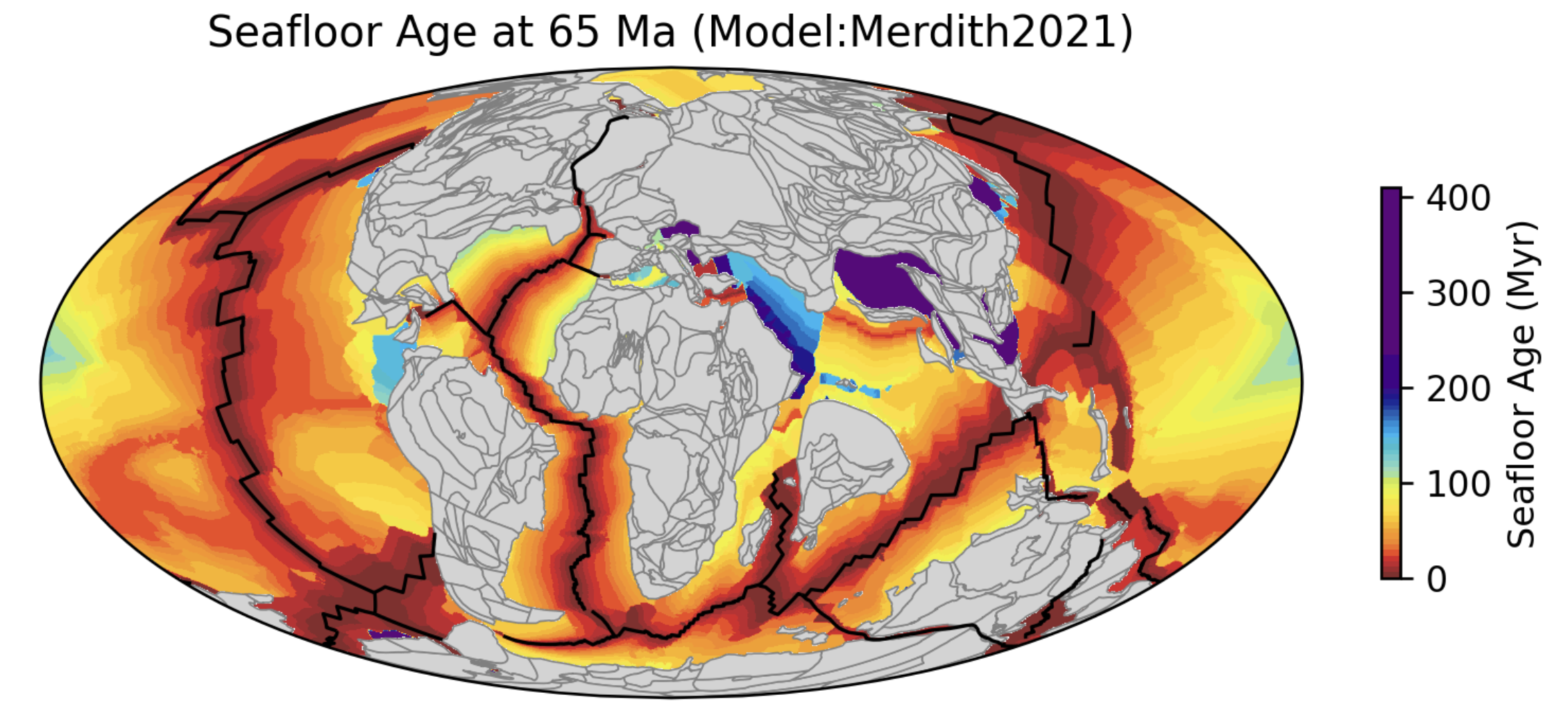
This notebook demonstrates how to generate seafloor age and spreading-rate grids through time. The figure below, generated by this notebook, shows seafloor age at 65 Ma. You may adjust the time parameter to generate grids at different geological times.

Citation:

Simon Williams, Nicky M. Wright, John Cannon, Nicolas Flament, R. Dietmar Müller, Reconstructing seafloor age distributions in lost ocean basins, Geoscience Frontiers, Volume 12, Issue 2, 2021, Pages 769-780, ISSN 1674-9871, https://doi.org/10.1016/j.gsf.2020.06.004.

import gplately

import glob, os
import matplotlib.pyplot as plt
import cartopy.crs as ccrs
from plate_model_manager import PlateModelManager

Define a rotation model, topology features and continents for the PlateReconstruction model

There are two ways to do this. To use local files, set use_local_files = True. To use PlateModelManager, set use_local_files = False.

use_local_files = False

1) Manually pointing to files

if use_local_files:
    # Method 1: manually point to files
    # you can download the model files at 
    # https://www.earthbyte.org/webdav/ftp/Data_Collections/Merdith_etal_2021_ESR/SM2-Merdith_et_al_1_Ga_reconstruction_v1.2.4.zip
    input_directory = "./SM2-Merdith_et_al_1_Ga_reconstruction_v1.2.4"
    
    rotation_model = glob.glob(os.path.join(input_directory, '*.rot'))
    static_polygons = input_directory+"/shapes_static_polygons_Merdith_et_al.gpml"
    topology_features = [
        input_directory+"/250-0_plate_boundaries_Merdith_et_al.gpml",
        input_directory+"/410-250_plate_boundaries_Merdith_et_al.gpml",
        input_directory+"/1000-410-Convergence_Merdith_et_al.gpml",
        input_directory+"/1000-410-Divergence_Merdith_et_al.gpml",
        input_directory+"/1000-410-Topologies_Merdith_et_al.gpml",
        input_directory+"/1000-410-Transforms_Merdith_et_al.gpml",
        input_directory+"/TopologyBuildingBlocks_Merdith_et_al.gpml"
        ]
    
    continents = input_directory+"/shapes_continents.gpml"
    coastlines = input_directory+"/shapes_coastlines_Merdith_et_al_v2.gpmlz"
    COBs =  None

    from pathlib import Path
    if not Path(input_directory).is_dir():
        raise FileNotFoundError(f"The input directory does not exist: {input_directory}. Ensure your files are in the correct locations or download the example input files at https://www.earthbyte.org/webdav/ftp/Data_Collections/Merdith_etal_2021_ESR/SM2-Merdith_et_al_1_Ga_reconstruction_v1.2.4.zip")
        

2) Using PlateModelManager

if not use_local_files:
    # Method 2: use PlateModelManager
    pm_manager = PlateModelManager()
    plate_model = pm_manager.get_model("Merdith2021", data_dir="plate-model-repo")
    
    rotation_model = plate_model.get_rotation_model()
    topology_features = plate_model.get_topologies()
    static_polygons = plate_model.get_static_polygons()
    
    coastlines = plate_model.get_layer('Coastlines')
    continents = plate_model.get_layer('ContinentalPolygons')
    COBs =  None
    

The SeafloorGrid object

...is a collection of methods to generate seafloor grids.

The critical input parameters are:

Plate model parameters

• PlateReconstruction_object: The gplately PlateReconstruction object defined in the cell below. This object is a collection of methods for calculating plate tectonic stats through geological time.
• PlotTopologies_object: The gplately PlotTopologies object defined in the cell below. This object is a collection of methods for resolving geological features needed for gridding to a certain geological time.

Define the PlateReconstruction and PlotTopologies objects

model = gplately.PlateReconstruction(rotation_model, topology_features, static_polygons)

gplot = gplately.PlotTopologies(model, continents=continents)

Time parameters

• max_time: The first time step to start generating age grids. This is the time step where we define certain gridding initial conditions, which will be explained below.
• min_time: The final step to generate age grids. This is the time when recursive reconstructions starting from max_time stop.

max_time = 410.
min_time = 65.

Ridge resolution parameters

With each reconstruction time step, mid-ocean ridge segments emerge and spread across the ocean floor. In gplately, these ridges are lines, or a tessellation of infinitesimal points. The spatio-temporal resolution of these ridge points can be controlled by two parameters:

• ridge_time_step: The "delta time" or time increment between successive resolutions of ridges, and hence successive grids. By default this is 1Myr, so grids are produced every millionth year.
• ridge_sampling: This controls the geographical resolution (in degrees) with which ridge lines are partitioned into points. The larger this is, the larger the spacing between successive ridge points, and hence the smaller the number of ridge points at each timestep. By default this is 0.5 degrees, so points are spaced 0.5 degrees apart.

ridge_time_step = 5. # We set the time step to 5 Myr to reduce the notebook’s runtime.
ridge_sampling = 0.5

---

Grid resolution parameters

The ridge resolution parameters mentioned above take care of the spatio-temporal positioning of ridge features/points. However, these ridge points need to be interpolated onto regular grids - separate parameters are needed for these grids.

For the max_time initial condition

At max_time, i.e. 410Ma, the PlateReconstruction model has not been initialised at 411Ma and any time(s) before that to sculpt the geological history before max_time. In terms of the workflow, all geological history before max_time is unknown. Thus, the global seafloor point distriubtion, and each point's spreading rate and age must be manually defined.

The initial point distribution is an icosahedral point mesh, made using stripy. This same mesh is used to create a continental mask per timestep, which is a binary grid that partitions continental regions from oceanic regions. Continental masks are used to determine which ocean points have collided/subducted into continental crust per timestep (these points are deleted from the seafloor grid at that timestep).

• refinement_levels: A unitless integer that controls the number of points in:

  • the max_time icosahedral point mesh, and
  • all continent masks.

  5 is the default. Any higher will result in a finer mesh.

• initial_ocean_mean_spreading_rate (in units of mm/yr or km/myr): Since the geological history before and at max_time is unknown, we will need to manually define the spreading rates and ages of all ocean points. This is manually set to a uniform spreading rate of 75 (mm/yr or km/myr). Each point's age is equal to its proximity to the nearest mid ocean ridge (assuming that ridge is the source of the point) divided by half this uniform spreading rate (half to account for spreading to the left and right of a ridge).

For the interpolated regular grids

The regular grid on which all data is interpolated has a resolution that can be controlled by:

• grid_spacing: The degree spacing between successive nodes in the grid. By default, this is 0.1 degrees. Acceptable degree spacings are 0.1, 0.25, 0.5, 0.75, or 1 degree(s) because these allow cleanly divisible grid nodes across global latitude and longitude extents. Anything greater than 1 will be rounded to 1, and anything between these acceptable spacings will be rounded to the nearest acceptable spacing.

refinement_levels = 6
initial_ocean_mean_spreading_rate = 50.

# Gridding parameter
grid_spacing = 0.25

extent=[-180,180,-90,90]

---

File saving and naming parameters

When grids are produced, they are saved to:

• save_directory: A string to a directory that must exist already.

These files are named according to:

• file_collection: A string used to help with naming all output files.

---

# continent masks, initial ocean seed points, and gridding input files are kept here
output_parent_directory = os.path.join(
    "NotebookFiles",
    "Notebook10",
)
save_directory = os.path.join(
    output_parent_directory,
    "seafloor_grid_output",
)
print(f"The ouput files created by this notebook will be saved in folder {save_directory}." )

# A string to help name files according to a plate model "Merdith2021"
file_collection = "Merdith2021"

The ouput files created by this notebook will be saved in folder NotebookFiles/Notebook10/seafloor_grid_output.

---

Subduction parameters

One of the ways an oceanic point can be deleted from the ocean basin at a certain timestep is if it is approaching a plate boundary such that a velocity and displacement test is passed:

Velocity test

First, given the trajectory of a point at the next time step, a point will cross a subducting plate boundary (and thus will be deleted) if the difference between its velocity on its current plate AND the velocity it will have on the other plate is greater than this velocity difference is higher than a specified threshold delta velocity in kms/Myr.

Displacement test

If the proximity of the point's previous time position to the plate boundary it is approaching is higher than a set distance threshold (threshold distance to boundary per Myr in kms/Myr), then the point is far enough away from the boundary that it cannot be subducted or consumed by it, and hence the point is still active.

The parameter needed to encapsulate these thresholds is:

• subduction_collision_parameters: This a tuple with two elements, by default (5.0, 10.0), for the (threshold velocity delta in kms/my, threshold distance to boundary per My in kms/my)

---

subduction_collision_parameters=(5.0, 10.0)

---

Methodology parameters

• resume_from_checkpoints: Gridding can take a couple of hours - if this is set to True and the routine is interrupted, rerunning the gridding cell will resume from where it left off, provided all files that have been saved before interruption have not been erased.
• zval_names: A list of strings to label the z-values we are gridding. By default, this is ['SPREADING_RATE'], because one z-value we are gridding is the spreading rate of all ocean points.

---

# Methodology parameters
resume_from_checkpoints = False,
zval_names = ['SPREADING_RATE']

Use all parameters to define SeafloorGrid:

# The SeafloorGrid object with all aforementioned parameters
seafloorgrid = gplately.SeafloorGrid(
    
    PlateReconstruction_object = model, 
    PlotTopologies_object = gplot, 
    
    # Time parameters
    max_time = max_time,
    min_time = min_time,
    
    # Ridge tessellation parameters
    ridge_time_step = ridge_time_step,
    ridge_sampling = ridge_sampling,
    
    # Gridding parameters
    grid_spacing = grid_spacing,

    extent = extent,
    
    # Naming parameters
    save_directory = save_directory,
    file_collection = file_collection,
    
    # Initial condition parameters
    refinement_levels = refinement_levels,
    initial_ocean_mean_spreading_rate = initial_ocean_mean_spreading_rate,
    
    # Subduction parameters
    subduction_collision_parameters = subduction_collision_parameters,
    
    # Methodology parameters
    resume_from_checkpoints = resume_from_checkpoints,
    zval_names = zval_names
)

How to use SeafloorGrid

1) Run seafloorgrid.reconstruct_by_topologies()

Running seafloorgrid.reconstruct_by_topologies() prepares all ocean basin points and their z-values for gridding, and reconstructs all active points per timestep to form the grids per timestep.

Initial conditions

At max_time, an initial ocean seed point icosahedral mesh fills the ocean basin. Each point is allocated a z-value, and this is stored in an .npz data frame at max_time. A netCDF4 continent mask is also produced at max_time.

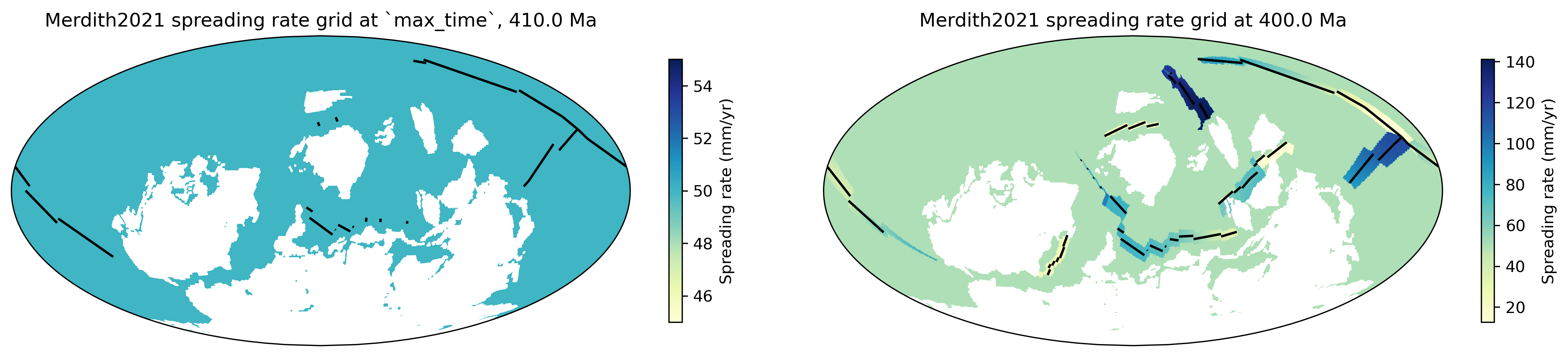
Below is an example of the initial condition: the ocean basin is populated with an intial_mean_ocean_spreading_rate of 50 mm/yr at a max_time of 410Ma. Reconstruction over 10Myr to 400Ma sees the points emerging from ridges with their own plate-model-ascribed spreading rates.

Preparing for gridding

At each successive timestep (ridge_time_step), new points emerge from spreading ridges, and they are allocated their own z-values. The workflow recursively outputs:

• 1 netCDF4 continent mask
• 1 GPMLZ file with point features emerging at spreading ridges (resolved according to the specified ridge_sampling)
• 1 .npz data frame for point feature z-values

for each time up to min_time. If the resume_from_checkpoints parameter is passed as True, and this preparation stage in seafloorgrid.reconstruct_by_topologies() is interrupted between max_time to min_time, you can rerun the cell. The workflow will pick up from where it left off provided all files that have been saved before interruption have not been erased.

To overwrite all files in save_directory (restart the preparation at max_time), pass resume_from_checkpoints as False. This happens by default.

Reconstruct by topologies

Once gridding preparation is complete, the ReconstructByTopologies object (written by Simon Williams, Nicky Wright, and John Cannon) in GPlately's reconstruct is automatically run. ReconstructByTopologies (RBT) identifies active points on the ocean basin per timestep. It works as follows:

If an ocean point on one plate ID transitions into another rigid plate ID at the next timestep, RBT calculates the point's velocity difference between both plates. The point may have subducted/collided with a continent at this boundary if this velocity difference is higher than a set velocity threshold. To ascertain whether the point should indeed be deactivated, a second test is conducted: RBT checks the previous time position of the point and calculates this point’s proximity to the boundary of the plate ID polygon it is approaching. If this distance is higher than a set distance threshold, then the point is far enough away from the boundary that it cannot be subducted or consumed by it and hence the point is still active. Else, it is deactivated/deleted.

Once all active points and their z-values are identified, they are written to the gridding input file (.npz) for that timestep.

import datetime
import time

start = time.time()
seafloorgrid.reconstruct_by_topologies()
end = time.time()
duration = datetime.timedelta(seconds=end - start)
print("Duration: {}".format(duration))

2) Run seafloorgrid.lat_lon_z_to_netCDF to write grids to netCDF

Calling seafloorgrid.lat_lon_z_to_netCDF grids one set of z-data per latitude-longitude pair from each timestep's gridding input file (produced in seafloorgrid.reconstruct_by_topologies()). Grids are in netCDF format.

The desired z-data to grid is identified using a zval_name. For example, seafloor age grids can be produced using SEAFLOOR_AGE, and spreading rate grids are SPREADING_RATE.

Use unmasked = True to output both the masked and unmasked versions of the grids.

seafloorgrid.lat_lon_z_to_netCDF("SEAFLOOR_AGE", unmasked=True)

seafloorgrid.lat_lon_z_to_netCDF("SPREADING_RATE", unmasked=True)

Plotting a sample age grid and spreading rate grid

Read one netCDF grid using GPlately's Raster object from grids, and plot it using the PlotTopologies object.

Notice the evolution of seafloor spreading rate from the initial value set with initial_ocean_mean_spreading_rate. Eventually, this initial uniform spreading rate will be phased out with sufficient recursive reconstruction.

time = min_time
# set the plot_unmasked_grid variable to True if you would like to see the unmasked age grid.
plot_unmasked_grid = False

# age grids
if not plot_unmasked_grid:
    agegrid_filename = f"{seafloorgrid.save_directory}/SEAFLOOR_AGE/{seafloorgrid.file_collection}_SEAFLOOR_AGE_grid_{time:0.2f}Ma.nc"
else:
    agegrid_filename = f"{seafloorgrid.save_directory}/SEAFLOOR_AGE/{seafloorgrid.file_collection}_SEAFLOOR_AGE_grid_unmasked_{time:0.2f}Ma.nc"

age_grid = gplately.grids.Raster(agegrid_filename)

# Prepare plots
fig = plt.figure(figsize=(8,4), dpi=240, linewidth=1)
ax = fig.add_subplot(111, projection=ccrs.Mollweide(central_longitude=20))

gplot.time = time
plt.title(f"Seafloor Age at {int(time)} Ma (Model:{seafloorgrid.file_collection})")

agegrid_cmap = "YlGnBu"
agegrid_cpt_file = "NotebookFiles/agegrid.cpt"
if not os.path.isfile(agegrid_cpt_file):
    print(f"The file {agegrid_cpt_file} does not exist locally. It can be found at https://raw.githubusercontent.com/GPlates/gplately/refs/heads/master/Notebooks/NotebookFiles/agegrid.cpt")
    print(f"The '{agegrid_cmap}' will be used to plot the age grid.")
    agegrid_cpt_file = None
if agegrid_cpt_file:
    try:
        from gplately.mapping.gmt_cpt import get_cmap_from_gmt_cpt
        agegrid_cmap=get_cmap_from_gmt_cpt(agegrid_cpt_file)
    except ImportError as e:
        print("To use GMT cpt file, ensure you are using GPlately version 2.1 or higher.")
        print(e)

im = gplot.plot_grid(
    ax, 
    age_grid.data, 
    cmap = agegrid_cmap,
    vmin = 0, 
    vmax =410,
)
gplot.plot_ridges(ax,linewidth=1)
if not plot_unmasked_grid:
    gplot.plot_continents(ax, edgecolor="grey", facecolor="lightgrey", linewidth=0.5)
plt.colorbar(im, label="Seafloor Age (Myr)", shrink=0.5, pad=0.05)

# Save figure
plt.savefig(
    f"{output_parent_directory}/{seafloorgrid.file_collection}_seafloor_age_{int(time)}Ma.png",
    bbox_inches = 'tight',
)

time = min_time
# set the plot_unmasked_grid variable to True if you would like to see the unmasked spreading rate grid.
plot_unmasked_grid = False

# spreading rate grids
if not plot_unmasked_grid:
    srgrid_filename = f"{seafloorgrid.save_directory}/SPREADING_RATE/{seafloorgrid.file_collection}_SPREADING_RATE_grid_{time:0.2f}Ma.nc"
else:
    srgrid_filename = f"{seafloorgrid.save_directory}/SPREADING_RATE/{seafloorgrid.file_collection}_SPREADING_RATE_grid_unmasked_{time:0.2f}Ma.nc"

sr_grid = gplately.grids.Raster(srgrid_filename)

# Prepare plots
fig = plt.figure(figsize=(8,4), dpi=240, linewidth=1)
ax = fig.add_subplot(111, projection=ccrs.Mollweide(central_longitude=20))

gplot.time = time
plt.title(f"Seafloor Spreading Rate at {int(time)} Ma (Model:{seafloorgrid.file_collection})")

spreading_rate_cmap = "magma"
spreading_rate_cpt_file = "NotebookFiles/spreading_full_rate.cpt"
if not os.path.isfile(spreading_rate_cpt_file):
    print(f"The file {spreading_rate_cpt_file} does not exist locally. It can be found at https://raw.githubusercontent.com/GPlates/gplately/refs/heads/master/Notebooks/NotebookFiles/spreading_full_rate.cpt")
    print(f"The '{spreading_rate_cmap}' will be used to plot the spreading rate grid.")
    spreading_rate_cpt_file = None
if spreading_rate_cpt_file:
    try:
        from gplately.mapping.gmt_cpt import get_cmap_from_gmt_cpt
        spreading_rate_cmap=get_cmap_from_gmt_cpt(spreading_rate_cpt_file)
    except ImportError as e:
        print("To use GMT cpt file, ensure you are using GPlately version 2.1 or higher.")
        print(e)

im = gplot.plot_grid(
    ax, 
    sr_grid.data, 
    cmap = spreading_rate_cmap,
    vmin = 0, 
    vmax =200,
)
gplot.plot_ridges(ax, linewidth=1)
if not plot_unmasked_grid:
    gplot.plot_continents(ax, edgecolor="grey", facecolor="lightgrey", linewidth=0.5)
plt.colorbar(im, label="Spreading rate (mm/yr)", shrink=0.5, pad=0.05, ticks=[0,50,100,150,200])

# Save figure
plt.savefig(
    f"{output_parent_directory}/{seafloorgrid.file_collection}_seafloor_spreading_rate_{int(time)}Ma.png",
    bbox_inches = 'tight',
)